2.20. Lecture 14: Agent-based models
Before this class you should:
Before next class you should:
Read Think Complexity, Chapter 10
Note Taker: Zain Siddiqui
2.20.1. Announcements
Approximately one month remains in the semester, so this is the final push for assignments and coursework.
Students are encouraged to sign up for System Thinkers presentations and review possible topics for inspiration.
Lab Test 2 is about one and a half weeks away. A lab tutor notebook will be released soon to assist with preparation.
Debate teams are currently being finalized.
2.20.2. Lab Test 2 Preparation
Students should review graph structures from Lectures 3 and 4.
Important concepts include clustering coefficient and average path length.
Regular Graph:
A regular graph has the following properties:
Every node has the same number of neighbours
High clustering coefficient
High average path length
Erdos-Renyi (Random) Graph:
In an Erdos-Renyi graph:
Each possible edge exists with probability \(p\)
Edges are placed randomly
Properties:
Low clustering coefficient (dependent on \(p\))
Low average path length due to random connectivity
Watts-Strogatz Graph:
The Watts-Strogatz model begins with a regular ring lattice and randomly rewires edges with probability \(p\).
Properties:
High clustering coefficient
Low average path length
Small World Example:
Milgram’s small-world experiment showed that letters required about six time steps on average to reach their destination.
This is evidence of the small-world property, which demonstrates that many real-world networks have short average path lengths.
2.20.3. Agent-Based Models
Agent-based models (ABMs) simulate systems using individual agents that follow simple rules.
Similar to cellular automata, ABMs are rule-based systems where complex behavior emerges from simple interactions.
Key characteristics include:
Agents represent individuals or entities
Agents gather information
Agents make decisions
Agents take actions
Agents typically operate in a space or network environment.
Local Information:
Agents usually operate with imperfect local information rather than full knowledge of the entire system.
This reflects the idea that agents do not have access to global information. Instead, they make decisions using only information from nearby agents or their local environment.
Example:
Job search platforms recommending opportunities based on previous activity and nearby information
Recommendation systems that suggest content based only on a user’s interactions
Randomness:
Agent-based models typically include randomness in agent behaviour and environmental conditions
Randomness helps simulate the unpredictability of the real world.
2.20.4. Applications of Agent-Based Models
Agent-based models are used in many fields.
- Finance:
ABMs can simulate financial systems. Examples include modeling interactions between high-frequency and low-frequency trading and analyzing how these interactions affect markets.
- Ecology:
Agent-based models are also used in ecological simulations and wildlife management studies.
- Crowd Simulation:
Pedestrian crowd models simulate how people move through public spaces.
Applications include:
Stadium design
Evacuation planning
Identifying congestion points
Poor crowd management has historically caused major stadium incidents, so these simulations are important for safety planning.
2.20.5. AI Agents
Artificial intelligence systems can also function as agents.
Examples include creating AI agents that:
Follow instructions
Process uploaded data
Optionally access internet resources
Examples include online AI agents and offline models such as OpenLLaMA.
2.20.6. Risks of AI Agents
Some potential issues include:
Hallucinated responses
Misuse of uploaded data
Incorrect evaluation of tasks
Example:
An AI grading agent incorrectly gave full marks to all submissions because it only compared characters rather than properly evaluating the answers. This demonstrates the importance of carefully designing agent rules.
2.20.7. Schelling’s Segregation Model
Thomas Schelling proposed a model of racial segregation.
Model Setup:
The city is represented as a grid
Each grid cell represents a house
Two types of agents occupy the houses
Approximately 10 percent of houses are empty
The agent satisfaction rule is that an agent is:
Happy if at least two neighbours are the same type
Unhappy otherwise
If an agent is unhappy, it moves to a randomly selected empty house.
Simulation Results:
Running the simulation leads to segregated clusters of agents.
Even though agents would tolerate mixed neighbourhoods, the system evolves toward homogeneous neighbourhoods.
If someone only observed the final state of the simulation, they might assume racism was the cause.
However, the model demonstrates that segregation can emerge from simple preferences rather than strong bias.
Real-world segregation may also be influenced by:
Employment opportunities
School systems
Crime levels
Wealth distribution
2.20.8. Schelling Model Implementation
The simulation can be implemented using a subclass of Cell2D.
Example structure:
class Schelling(Cell2D):

    def __init__(self, n, p):
        self.p = p
        choices = np.array([0, 1, 2], dtype=np.int8)
        probs = [0.1, 0.45, 0.45]
        self.array = np.random.choice(choices, (n, n), p=probs)

        self.options = dict(mode='same', boundary='wrap')

        self.kernel = np.array([[1, 1, 1],
                                [1, 0, 1],
                                [1, 1, 1]], dtype=np.int8)
        num_red = correlate2d(red, self.kernel, **self.options)
        num_blue = correlate2d(blue, self.kernel, **self.options)
        num_neighbors = num_red + num_blue
Simulation Steps:
Identify unhappy agents
Select an empty location
Move the agent
Repeat until equilibrium (no agents remain unhappy and no further moves occur)
Example logic of Step Function:
num_empty = np.sum(empty)

for source in unhappy_locs:
    i = np.random.randint(num_empty)
    dest = empty_locs[i]

    a[dest] = a[source]
    a[source] = 0
    empty_locs[i] = source
2.20.9. Simulation Observations
When the model runs:
Most segregation occurs early in the simulation
Later steps produce smaller changes
- Example result:
If \(p = 0.3\), approximately 75 percent of agents become happy.
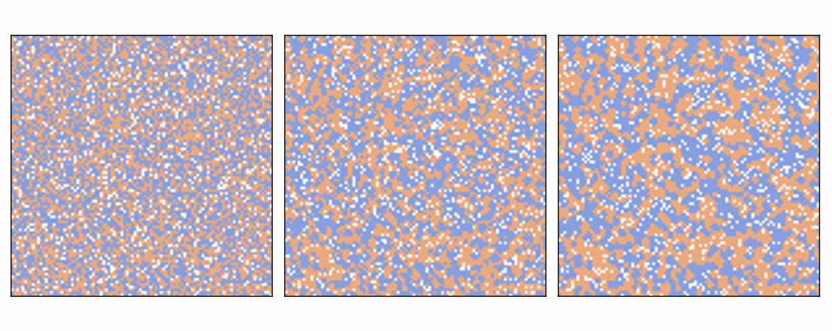
Example simulation showing segregation clusters forming over time.
2.20.10. Sugarscape Model
In 1996, Joshua Epstein proposed the Sugarscape model. Sugarscape is an artificial society simulation used to study economic and social systems.
Agents move on a two-dimensional grid representing a landscape. Each cell has a maximum sugar capacity.
In the original configuration:
Center cells have capacity 4
Surrounding rings have capacities 3, 2, and so on
Agent Attributes:
Each agent has three attributes.
- Sugar:
Random value in range \([5,25]\)
- Metabolism:
Uniform distribution \([1,4]\)
- Vision:
Uniform distribution \([1,6]\)
Agent Behaviour:
Each agent performs the following steps:
Observe cells within its vision range
Choose the unoccupied cell with the most sugar
Move to that location
Consume sugar according to its metabolism
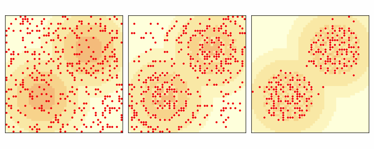
Sugarscape environment with different sugar capacities.
2.20.11. Emergent Patterns
The Sugarscape simulation produces several emergent behaviours as agents interact with their environment and compete for resources.
Agents with higher vision:
Move toward higher-resource areas quickly
Deplete resources rapidly
Create migration waves
These patterns resemble spaceship movements observed in cellular automata.
Wealth Distribution:
The distribution of sugar among agents can produce wealth inequality.
This inequality emerges naturally from the simulation rather than being explicitly programmed.
2.20.12. Emergence
An emergent property is a system-level behaviour that arises from the interaction of components.
Examples from this lecture include:
- Segregation:
Emerges from individual movement rules
- Wealth distribution:
Emerges from resource consumption patterns
- Migration waves:
Emerges from agent movement and vision
Emergent behaviours show us how simple local rules can produce complex global outcomes.
2.20.13. Attribution
Downey, A. Think Complexity, 2nd Edition