2.18. Lecture 12: Physical modelling
Before this class you should:
Read Think Complexity, Chapter 7, and answer the following questions:
What is diffusion? What is reaction diffusion?
How does cellular automata relate to diffusion?
What is percolation? What exactly are porous cells?
How would you use cellular automata to simulate physical systems?
What is cross correlation and convolution? How can we use these to define diffusion?
Form a project team and choose a topic
Before next class you should:
Read Think Complexity, Chapter 8
Note Taker: Syed Uzair Ali
2.18.1. Overview
Introduced physical modelling, focusing on how simple local rules can approximate real-world processes
Two real-life models discussed, diffusion and percolation
Diffusion models simulate how a chemical spreads across a grid
Percolation models simulate the movement of a fluid through porous material
Talked about physical phenomena and how they relate to phase transition and fractal patterns
2.18.2. Administrative Notes
Upcoming deliverables:
System thinkers presentation (Due March 18)
Group project (Initial idea and group due March 11)
Lab Test 2 (Week of March 19)
2.18.3. From Discrete to Continuous Models
In the previous lecture, we discussed Conway’s Game of Life.
Up to this point, the cellular automata we studied used discrete states. However, many simple cellular automata are insufficient to describe real-world physical phenomena.
Some cellular automata are intended as physical models. While patterns such as beehives or toads in the Game of Life are emergent structures, they are not physical models of natural processes.
We shift toward continuous-state models in two dimensions that approximate real-world behaviour.
2.18.4. Physical Modelling
Physical models are designed to represent real phenomena.
Two examples discussed in this lecture:
Chemical diffusion
Percolation of a liquid
These systems can exhibit complex behaviour and fractal geometry.
2.18.5. Turing and Morphogenesis
In 1952, Alan Turing published The Chemical Basis of Morphogenesis.
Turing demonstrated that patterns can arise from a homogeneous state. His work was based on differential equations describing chemical reactions and diffusion.
In his paper, he showed that reaction–diffusion systems could produce spatial patterns through local interactions.
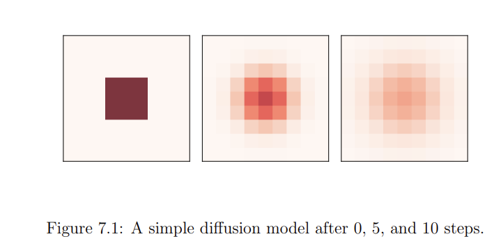
2.18.6. Diffusion Model (Single Chemical)
We first consider the diffusion of a single chemical.
Rules:
Each cell contains a value between \(0\) and \(1\) representing concentration.
If concentration exceeds that of neighbouring cells, chemical flows outward.
If concentration is lower than neighbours, chemical flows inward.
The process continues until equilibrium is reached, meaning concentration is uniform.
The code block below shows the kernel used to correlate with the concentration grid.
kernel = np.array([[0, 1, 0],
                   [1,-4, 1],
                   [0, 1, 0]])

c = correlate2d(array, kernel, mode='same')
array += r * c
2.18.7. Reaction–Diffusion Model (Two Chemicals)
The Reaction-Diffusion Model is another type of diffusion model in which there are two elements diffusing We now introduce two interacting chemicals, \(A\) and \(B\). This is different than the previous example as now instead of one, theres two chemicals interacting
Parameters:
Diffusion rate of \(A\) ( \(r_a\) )
Diffusion rate of \(B\) ( \(r_b\) )
Feed rate ( \(f\) )
Kill rate ( \(k\) )
In many models, \(r_b\) is approximately half of \(r_a\).
The feed rate controls how quickly \(A\) is added.
The kill rate controls how quickly \(B\) is removed.
The reaction term is:
Update equations:
These equations can be used as seen below in the code block.
class ReactionDiffusion(Cell2D):
   def __init__(self, n, m, params, noise=0.1):
   self.params = params
   self.array = np.ones((n, m), dtype=float)
   self.array2 = noise * np.random.random((n, m))
   add_island(self.array2)

def step(self):
   A = self.array
   B = self.array2
   ra, rb, f, k = self.params

   cA = correlate2d(A, self.kernel, **self.options)
   cB = correlate2d(B, self.kernel, **self.options)

   reaction = A * B**2
   self.array += ra * cA - reaction + f * (1-A)
   self.array2 += rb * cB + reaction - (f+k) * B
Despite having only four parameters, this system produces complex spatial patterns as seen below.
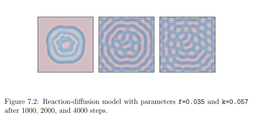
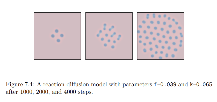
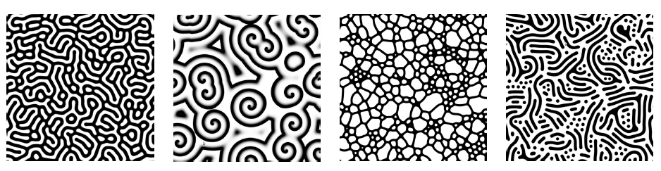
With this model, behaviours similar to biological processes such as cell division (mitosis-like splitting) can emerge.
This can occur when:
Regions with high concentration of \(A\) and low concentration of \(B\) become unstable and split into separate regions.
Areas where \(B\) rapidly reacts with \(A\) (through the \(AB^2\) reaction term) consume \(A\), creating boundaries between regions.
These interactions between reaction and diffusion allow patterns to grow, divide, and form complex structures.
2.18.8. Percolation
Percolation describes fluid movement through a porous medium.
Examples:
Oil moving through rock
Water spreading through paper
Percolation theory also applies to:
Epidemics
Resistor networks
We focus on a two-dimensional cellular automaton model.
2.18.9. Percolation Rules
This implementation uses a von Neumann neighborhood where diagonals are not included.
Each cell is porous with probability \(q\), otherwise it is non-porous.
All cells start dry except the top row, which is wet.
At each time step, a porous cell becomes wet if it has at least one wet neighbour.
Non-porous cells remain dry.
The simulation continues until a fixed point is reached.
Below is the code block to represent the percolation model.
class Percolation(Cell2D):
   def __init__(self, n, q):
   self.q = q
   self.array = np.random.choice([1, 0], (n, n), p=[q, 1-q])
   self.array[0] = 5

kernel = np.array([[0, 1, 0],
                   [1, 0, 1],
                   [0, 1, 0]])

def step(self):
   a = self.array
   c = correlate2d(a, self.kernel, mode='same')
   self.array[(a==1) & (c>=5)] = 5
If a connected path of wet cells spans from the top to the bottom row, the system contains a percolating cluster.
The model can be tested to see if it contains a cluster through the code below. It returns true if any of the bottom row cells are wet, indicating that there is a cluster present.
def test_perc(perc):
   num_wet = perc.num_wet()
   while True:
   perc.step()

   if perc.bottom_row_wet():
      return True
   new_num_wet = perc.num_wet()

   if new_num_wet == num_wet:
      return False

   num_wet = new_num_wet
2.18.10. Critical Phenomena and Phase Transitions
A phase transition is when a small change in a system parameter causes a sudden change in the global behavior of a system.
A common example is when water changes phases, such as from liquid to solid when the temperature exceeds a certain point.
The following code uses a random walk where it tests a range of q values and checks whether the grid has a percolating cluster.
It returns a list of q values which can then be averaged to get a “critical probability”
At the critical probability \(q_c\), is where the system undergoes a phase transition.
At criticality, systems exhibit something known as fractal geometry which is discussed in the next section.
2.18.11. Fractals and Fractal Geometry
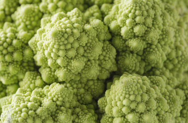
Fractals are geometric structures that exhibit self-similarity, meaning their pattern repeats at different scales. For example, zooming into a fractal will resemble the overall object.
This image below shows how fractals are found in nature, in this case Romanesco broccoli.
Mathematically, fractals relate to scaling behaviour and non-integer dimensions.
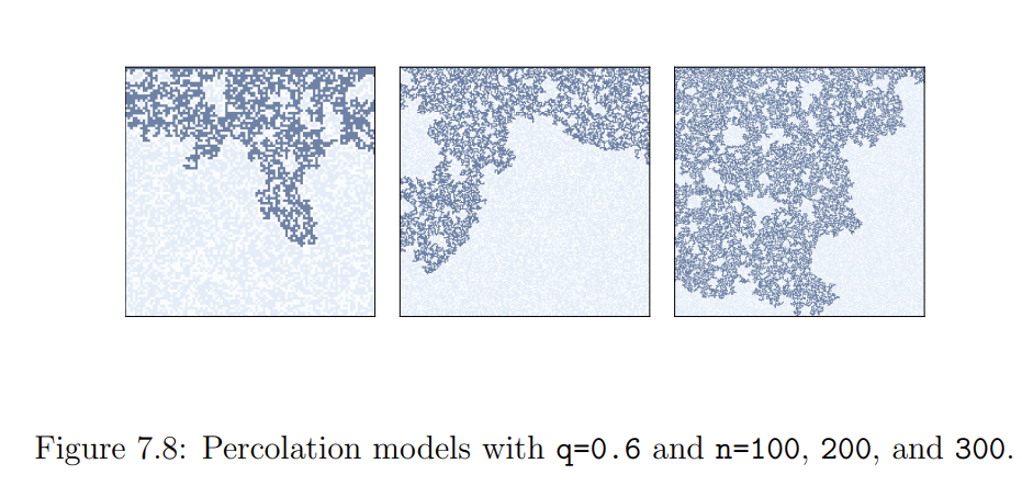
Large systems near the critical value produce complex, self-similar structures.
Combining fractal geometry with critical phenomena, we can get interesting results when we run percolation models at critical values for large n values. Seen by the image below, the percolation model exhibits fractal geometry, in which no matter the scale, the pattern is the same.
2.18.12. Attribution
Karl Sims, Reaction–Diffusion tutorial: http://karlsims.com/rd.html
Downey, A. Think Complexity, 2nd Edition