2.10. Lecture 9: Scale-free networks

Before this class you should:

• Read Think Complexity, Chapter 4, and answer the following questions:

  1. The probability mass function (PMF) plotted in Figure 4.1 is a normalized version of what other kind of plot?

  2. What is the continuous analogue of the PMF?

Before next class you should:

• Read Think Complexity, Chapter 5

Note taker: Sofia Rimando

2.10.1. Overview

• Compared real Facebook network data to generative models

• Reviewed the Watts–Strogatz (WS) model

• Introduced degree distributions

• Discussed heavy-tailed and power law distributions

• Introduced the Barabási–Albert (BA) generative model

• Compared WS and BA models using clustering, path length, and degree

• Introduced cumulative distribution functions (CDF and CCDF)

• Discussed explanatory models in complexity science

2.10.2. Ego Networks

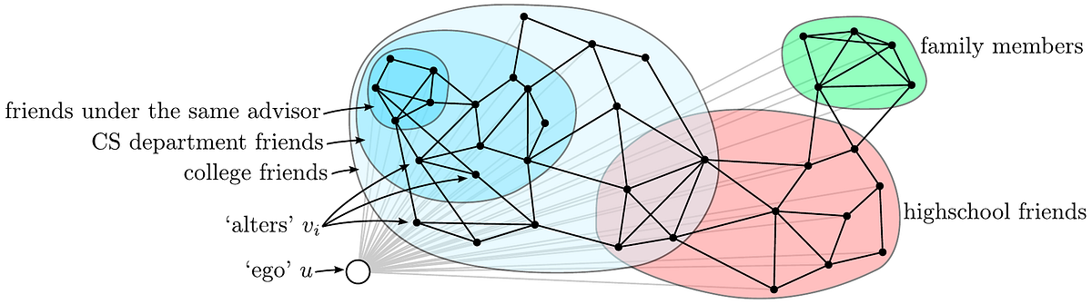
An ego network consists of a focal node (the “ego”), the nodes directly connected to it (the “alters”), and the connections among those alters.

This structure focuses on a local portion of a larger social network.

In social network analysis:

• The ego is the central individual.

• Alters are immediate neighbours.

• Edges among alters reveal clustering within the ego’s community.

Ego networks allow researchers to study:

• Community structure

• Overlapping circles

• Local clustering behaviour

In this lecture, ego networks serve as an entry point for analyzing large-scale social graphs. The following is an example of an ego network [1]:

2.10.3. SNAP Facebook Dataset

The dataset used in this chapter comes from the Stanford Network Analysis Project (SNAP) [2]. It contains Facebook friendship data with:

• 4039 users (nodes)

• 88,234 friendships (edges)

Each edge represents a mutual friendship.

The goal is to determine whether this network exhibits small-world properties including:

1. High clustering coefficient

2. Short average path length

Because the dataset is large, approximate algorithms are used.

The clustering coefficient is estimated using the NetworkX approximation function average_clustering from networkx.algorithms.approximation, which provides an efficient estimate for large graphs. The average path length is estimated by sampling random node pairs.

Results:

1. Average clustering coefficient ≈ 0.61

2. Average path length ≈ 3.7

These values indicate that the Facebook network exhibits small-world behaviour: strong local clustering and short average separation between users. To understand how such structure can arise, generative network models are examined to assess whether they reproduce these properties.

2.10.4. Watts–Strogatz Model

A Watts–Strogatz (WS) graph is a generative network model designed to capture small-world structure observed in many real networks. The model begins with a regular ring lattice where each node is connected to its \(k\) nearest neighbours. Each edge is then rewired with probability \(p\), introducing randomness while preserving local connectivity.

The parameter \(p\) controls the level of randomness in the network:

• \(p = 0\) produces a ring lattice with high clustering and long paths

• \(p = 1\) produces a random graph with low clustering and short paths

• Intermediate values of \(p\) yield small-world networks with both high clustering and short average path length

To model the Facebook network, a WS graph is constructed:

n = len(fb)
m = len(fb.edges())
k = int(round(2*m/n))

Here, \(k\) represents the average degree.

Ring lattice (\(p = 0\))

• Clustering ≈ 0.73

• Path length ≈ 46

Random graph (\(p = 1\))

• Clustering ≈ 0.01

• Path length ≈ 2.6

Intermediate case (\(p = 0.05\))

• Clustering ≈ 0.63

• Path length ≈ 3.2

The WS model with \(p = 0.05\) reproduces the small-world characteristics of the Facebook data.

The WS model captures clustering and short paths, but social networks also display significant variation in node degree. To determine whether the model reproduces this pattern, the degree distribution is examined.

2.10.5. Degree

The degree of a node is the number of edges connected to it.

def degrees(G):
    return [G.degree(u) for u in G]

Mean degree:

• Facebook ≈ 43.7

• WS ≈ 44

Standard deviation:

• Facebook ≈ 52.4

• WS ≈ 1.5

Although the mean degrees are similar, the WS model produces nearly uniform degrees, while the Facebook data shows extreme variability. This can be examined by graphing the probability mass function (PMF):

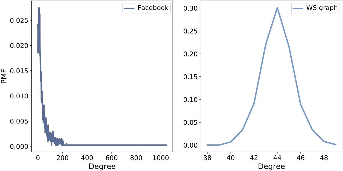
PMF of node degree for Facebook data and the WS model. The WS distribution is tightly concentrated, while the Facebook distribution shows large variability.

2.10.6. Heavy-Tailed Distributions

A heavy-tailed distribution is one in which extreme values occur more frequently than expected under a normal distribution. This implies a non-negligible probability of observing values far from the mean.

The Facebook degree distribution contains:

• Many users with few friends

• A small number of users with extremely many friends

As such, the Facebook data exhibits a heavy-tailed distribution.

If a distribution follows a power law, taking logarithms of both the variable and probability transforms the relationship into a linear form. Therefore, plotting the distribution on log-log axes allows the visual detection of power law behaviour through an approximately straight tail.

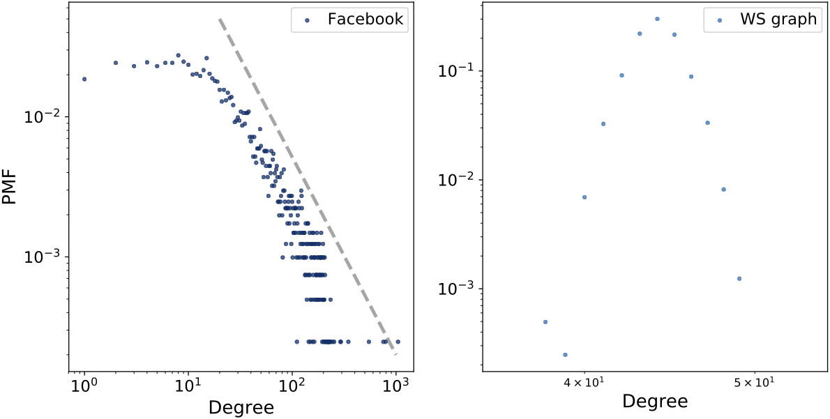
The log-log plot of the Facebook degree distribution illustrates the approximately linear tail characteristic of power law behaviour.

A power law has the form:

\[PMF(k) \sim k^{-\alpha}\]

Taking the logarithm:

\[\log PMF(k) \sim -\alpha \log k\]

On a log-log plot, this produces a straight line with slope \(-\alpha.\)

The WS model does not reproduce this behaviour.

2.10.7. Barabási–Albert Model

Barabási and Albert proposed a generative model that produces scale-free networks.

The BA model differs from WS in two major ways.

Growth: The network begins with a small graph and adds nodes one at a time.

Preferential attachment: New nodes are more likely to connect to nodes that already have many edges. This produces hubs and a “rich get richer” effect.

A BA network is generated using the NetworkX function barabasi_albert_graph, which takes parameters \(n\) and \(m\). Here, \(n\) denotes the number of nodes in the network and \(m\) is the number of edges each newly added node forms through preferential attachment.

To generate a BA network with comparable size and mean degree to the Facebook dataset, the model can be constructed by

ba = nx.barabasi_albert_graph(n=4039, m=22)

Here, \(n\) specifies the number of generated nodes and \(m\) controls the number of edges each new node creates when it joins the network.

Results:

• Mean degree ≈ 43.7

• Standard deviation ≈ 40.1

• Path length ≈ 2.5

• Clustering ≈ 0.037

The BA model captures the heavy-tailed degree distribution much better than WS, but it fails to reproduce high clustering.

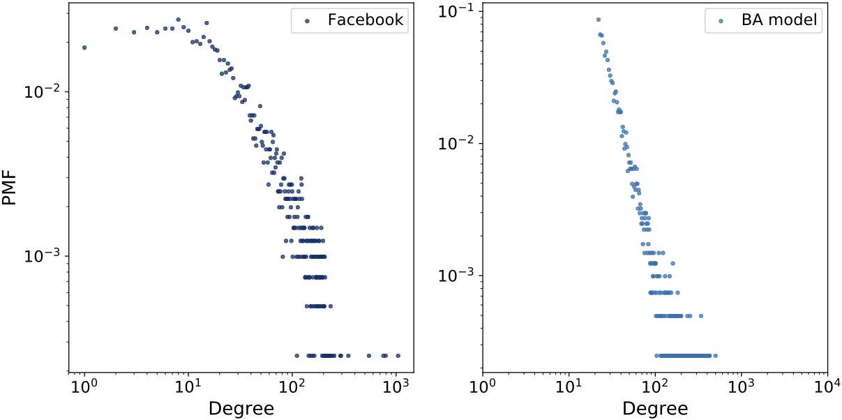
Log-log comparison of degree distributions for Facebook data and the BA model. The BA model better captures the heavy tail.

2.10.8. Model Comparison

	Facebook	WS Model	BA Model
Clustering	0.61	0.63	0.037
Path length	3.69	3.23	2.51
Mean degree	43.7	44	43.7
Std degree	52.4	1.5	40.1

The WS model captures clustering and path length but fails to reproduce the heavy-tailed degree distribution, whilst the BA model captures heavy-tailed degree behaviour and short paths but fails to reproduce the high clustering observed in the data.

2.10.9. Cumulative Distributions

PMFs can be noisy in the tail. A cumulative distribution function (CDF) gives the probability that a random variable is less than or equal to a given value, and thus provides a smoother representation.

Definition:

\[CDF(x) = P(X \le x)\]

Complementary CDF:

\[CCDF(x) = 1 - CDF(x)\]

If the distribution follows a power law:

\[CCDF(x) \sim x^{-\alpha}\]

On a log-log scale, the CCDF appears linear in the tail.

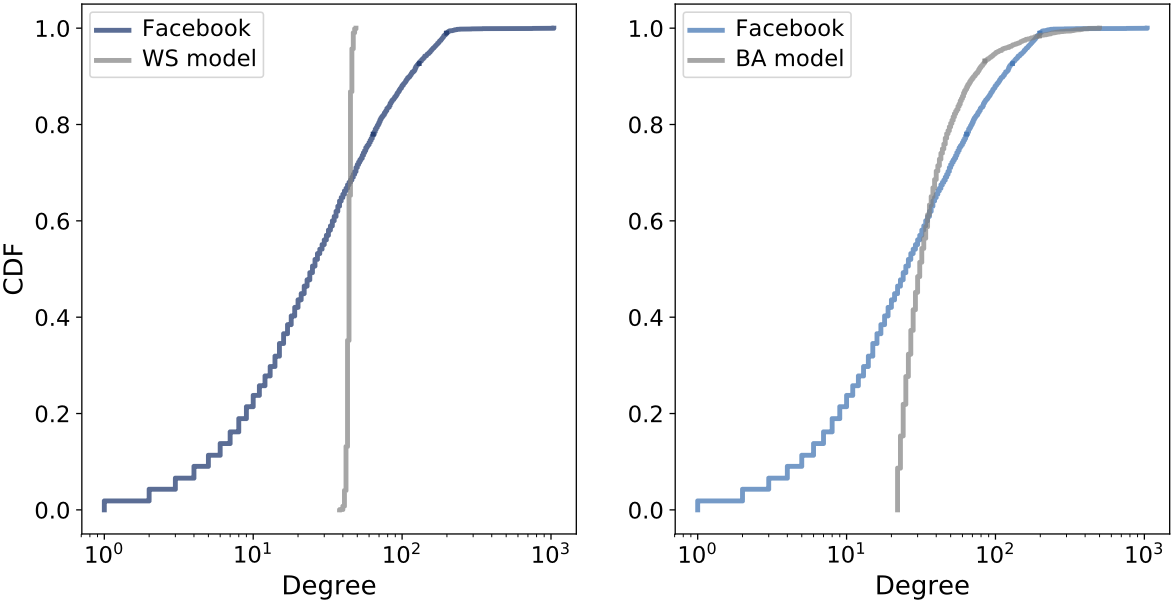
CDF of degree on a log-x scale (left), and complementary CDF on a log-log scale (right). Linear tail behaviour suggests approximate power law structure.

2.10.10. Explanatory Models

An explanatory model attempts to answer the question “Why?”

Structure:

1. Observe a phenomenon in a real system.

2. Construct an analogous model.

3. If the model reproduces the phenomenon, it provides an explanation.

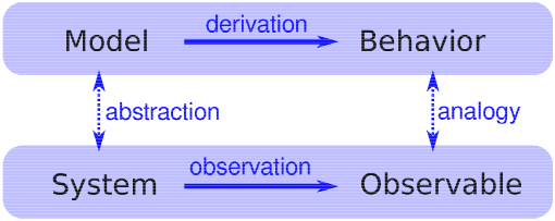
Logical structure of an explanatory model. A model is constructed to represent important features and characteristics of a system and is evaluated based on its ability to reproduce observed phenomena [3].

WS explanation: Short paths arise from weak ties connecting clustered groups.

BA explanation: Short paths arise from hubs formed through preferential attachment.

Neither model is perfect. Each explains different aspects of the Facebook network. This demonstrates a central idea in complexity science: different models explain different features of the same system.

2.10.11. References

[1]

ResearchGate. “Ego network with labelled social circle.” Available at: https://www.researchgate.net/figure/Ego-network-with-labelled-social-circle_fig1_348049269

[2]

Stanford Network Analysis Project (SNAP). https://snap.stanford.edu/

[3]

Allen B. Downey, Think Complexity online HTML edition. Available at: https://greenteapress.com/complexity/html/thinkcomplexity.html