3.2. Lab 1: Scientific Python

Due Date: 11:59pm January 28, 2024 Labs should be submitted as a single Jupyter notebook to CourseLink Dropbox This lab counts for 4% of the final grade

To do in advance of this lab:

• Set up the scientific Python tools as explained in Computing Resources.

• Attend the Lab Session where the TAs presented NumPy, Matplotlib and Scipy. If you would like to review further att your own pace, you can work through the following sections of “Getting Started” in the Scipy Lecture Notes:

  • 1.4 NumPy: creating and manipulating numerical data

  • 1.5 Matplotlib: plotting

  • 1.6 Scipy : high-level scientific computing

  If you are new to Python, you should budget 2-3 hours to go through all of this material. If you are comfortable with the TAs’ presentation, then feel free to dive right into this lab and refer to Scipy Lecture Notes as needed.

3.2.1. Background

In this lab, we will create a model of how a hot cup of tea cools down once the liquid has been poured into a cup.

Source: This example has been adapted from the University of Southampton’s Scientific Python Training Program with credit to Hans Fangohr and the rest of the teaching staff.

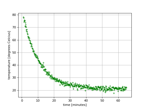
A research team has measured the temperature of a cooling cup of tea using some specialized equipment.

(Source code, png, hires.png, pdf)

The equipment takes one temperature reading every 10 seconds. The measurements are noisy, and something also went wrong with the equipment such that no data was collected for the first minute.

3.2.2. Research questions

The questions we aim to answer are:

1. What was the initial temperature (at \(t=0\))?

2. How quickly does the tea cool down? In particular, at what time is it safe to drink (assuming a safe temperature is 60 deg C)?

3. What will be the final temperature of the tea if we wait indefinitely (presumably this will be the temperature of the room where the experiment was conducted)?

3.2.3. Strategy

To make progress, let’s make a few simplifying assumptions and define some variables:

• We assume that the initial temperature, \(T_i\), is the temperature at which the tea has been poured into the cup.

• If we wait indefinitely, the final temperature will reach the value of the ambient temperature, \(T_a\), which will be the environmental temperature in the lab where the measurements were taken.

• We further assume that the cup has no significant heat capacity to keep the problem simple.

• We assume that the cooling process follows a particular model. In particular, we assume that the rate with which the temperature \(T\) changes as a function of time is proportional to the difference between the current temperature \(T(t)\) and the temperature of the environment \(T(a)\):

  \[\frac{dT}{dt} = \frac{1}{C} \left( T_a - T \right)\]

  We can solve this differential equation analytically and obtain a model equation:

  (1)\[T(t) = \left( T_i - T_a \right) \exp \left( \frac{-t}{C} \right) + T_a\]

  where \(C\) is the time constant for the cooling process (which is expressed in seconds). The larger \(C\), the longer it takes for a hot drink to cool down. Over a period of \(C\) seconds, the drink’s temperature will decrease by roughly 2/3.

3.2.4. Preparation

Create a Jupyter notebook and implement a function model(t, Ti, Ta, C) which implements Equation (1).

3.2.4.1. Examples

In [1]: model(0, 100, 0, 10)
Out[1]: 100.0

In [2]: model(10, 100, 0, 10)
Out[2]: 36.787944117144235

In [3]: model(10, 100, 100, 10)
Out[3]: 100.0

In [4]: model(1000000, 100, 25, 10)
Out[4]: 25.0

The function model(t, Ti, Ta, C) should return a single value if \(t\) is a floating point number, and an array if \(t\) is an array. For example:

In [5]: model(0, 100, 20, 500)
Out[5]: 100.0

In [6]: ts = np.linspace(0, 3600, 4)


In [7]: ts
Out[7]: array([    0.,  1200.,  2400.,  3600.])

In [8]: model(ts, 100, 20, 500)
Out[8]: array([ 100.        ,   27.25743626,   20.65837976,   20.05972686])

Now is the time to seek help from the lab team if you are having any difficulties. Make sure your model function is correct before moving on.

3.2.5. Assessment

Unfortunately the research team saved their data in Matlab format and you must figure out a way to read it in Python. Here is their Matlab file containing the data (click the Download button once you reach the GitHub page).

Suddenly you remember reading in the Scipy Lecture Notes something about the functionality to read Matlab files in Python. The Matlab file contains a single array called data. Read this into a NumPy array. It should be 385 rows (the measurements) by 2 columns. The first column contains the timestamp in seconds and the second column contains the temperature reading.

Add a function extract_parameters(ts, Ts) to your notebook which expects a numpy array ts with time values and a numpy array Ts of the same length as ts with corresponding temperature values. The function should estimate and return a tuple of the three model parameters Ti, Ta and C (in this order) by fitting Equation (1) to the data ts and Ts.

Hint: You should use the curve_fit function from Scipy. It may need some initial guesses (through the optional function parameter p0) for the model parameters to find a good fit.

Add a function sixty_degree_time(Ti, Ta, C) which expects the model parameters Ti (initial temperature), Ta (ambient temperature) and C (the cooling rate time constant). The function should return an estimate of the number of seconds after which the temperature of the tea has cooled down to 60 degrees Celsius.

Hint: You have at least two different possible ways of obtaining this number of seconds for a given set of model parameters (Ti, Ta, C). One involves a root finding algorithm. You can assume that Ti > 60 degrees Celsius, and that Ti > Ta.

Please submit a Jupyter notebook which includes the following functions:

• model

• extract_parameters

• sixty_degree_time

It should also include a plot of your fitted curve, and clearly answer each of the “Research Questions” posed above.